About
Demodulation with a Simple Analog Circuit
1. Circuit Implementation
Building a Resolver Observer
1. Speeding Up with Theory
Handling Imperfect Parameters
Rotation Multiples
Conclusion

About

Resolvers are a sensor commonly used to measure the angle of an electric motor. The purpose of this page is to cover some different problems I have had to tackle related to resolvers, including some less than ideal scenarios.

Section 2 goes over a solution to demodulate the resolver signals using a simple analog circuit. Section 3 walks through deriving a resolver observer or tracker. Sections 4 and 5 handle some imperfections that may occur with resolvers such as dealing with unknown parameters and dealing with weird rotation multiples.

To provide only a very basic description for context, a resolver takes in a carrier signal and returns a modulated sine and cosine signals. These signals are a combination of both the carrier signal and information about the position. The position information is encoded in the envelope of the modulated signal. Some sort of demodulation method is needed to remove the carrier signal. From the demodulated signals, the position has to be estimated, along with any other position derivatives. Scaling may also be needed to translate from resolver reported position to the position which is actually desired.

Demodulation with a Simple Analog Circuit

The signals from the resolver are plotted below. The carrier signal is driven into one pair of terminals on the resolver, and the outputs on the other terminal pairs are the modulated sine and modulated cosine signals. As the shaft moves, the envelope of the sine and cosine signals change with angle.

A function model for the modulated signals is

\[C = \sin(2\cdot\pi\cdot f_c \cdot t) \] \[V_{sin} = C \cdot \sin(\theta)\] \[V_{cos} = C \cdot \cos(\theta) \]

The desired output signals are only the \(\sin(\theta)\) and \(\cos(\theta)\) parts. There are many ways to perform this extraction, but a very simple method is

Multiplying each modulated signal against the carrier signal
Apply low pass filtering to the product

There are a few reasons why this works. A very simple one is that "multiplication in the time domain is addition in the frequency domain." When applied to this scenario, the carrier signal and demodulated signals both contain content at \(\pm f_c\). By multiplying the signals together in the time domain, in the frequency domain this would create content at \(0\) and \(\pm 2 f_c\). By applying low pass filtering, the \(\pm 2 f_c\) terms can be made small, leaving just the near-0 frequency term which corresponds to the rotational frequency.

The following Julia code shows this in practice. A note is that the demodulated signal needs to be multiplied by 2 to achieve the correct envelope signal. This is related to the fact that the carrier and modulated signals have a magnitude of \(0.5\) at \(\pm f_c\), instead of 1.

using ModelingToolkit, OrdinaryDiffEq, Plots
using DataInterpolations, Distributions
gr()
using ModelingToolkit: t_nounits as t, D_nounits as D

shaft_speed = 1000
num_cyc = 2.5
Ts = 1e-5
per = num_cyc * (2*pi/shaft_speed)

@variables begin
    carrier(t)
    we(t)
    theta(t)
    sine_sig(t)
    cosine_sig(t)
    muxed_sine(t)
    muxed_cosine(t)
    demodded_sine(t)
    demodded_cosine(t)
    est_theta(t)
end
@parameters begin
    carrier_freq = 10e3
end

@mtkcompile mod_resolver = System(Equation[
    we ~ shaft_speed
    D(theta) ~ we
    carrier ~ sin(carrier_freq * 2 * pi * t)
    sine_sig ~ sin(theta) * carrier
    cosine_sig ~ cos(theta) * carrier
    muxed_sine ~ sine_sig * carrier
    muxed_cosine ~ cosine_sig * carrier
    D(demodded_sine) ~ (2*muxed_sine - demodded_sine) * 2 * pi * (carrier_freq/5)
    D(demodded_cosine) ~ (2*muxed_cosine - demodded_cosine) * 2 * pi * (carrier_freq/5)
    est_theta ~ atan(demodded_sine, demodded_cosine)
], t)

u0 = [
    mod_resolver.theta => 0.0
    mod_resolver.demodded_sine => 0.0
    mod_resolver.demodded_cosine => 1.0
]

prob = ODEProblem(mod_resolver, u0, (0, per))
sol = solve(prob, Tsit5(), saveat=Ts)

p_pos = plot(sol[t], mod.(sol[mod_resolver.theta], 2*pi), label="Ang")
plot!(p_pos, sol[t], mod.(sol[mod_resolver.est_theta], 2*pi), label ="Est Ang")

pos_err = mod.(sol[mod_resolver.theta] .- sol[mod_resolver.est_theta] .+ pi,
    2*pi) .- pi

p_car = plot(sol[t], sol[mod_resolver.carrier], label="Carrier")

p_sine = plot(sol[t], sol[mod_resolver.sine_sig], label="Modulated sine")
plot!(p_sine, sol[t], sol[mod_resolver.demodded_sine], label="Demodulated sine")

p_cosine = plot(sol[t], sol[mod_resolver.cosine_sig], label="Modulated cosine", 
    xlabel="Time [s]")
plot!(p_cosine, sol[t], sol[mod_resolver.demodded_cosine], label="Demodulated cosine")

plot(p_pos, p_car, p_sine, p_cosine, layout=(4,1), legend=:right)

To further drive the point home, here are the FFT plots of the various signals, including negative frequencies.

using FFTW, LaTeXStrings
function calc_fft(Ts, data)
    N = length(data)
    Fs = 1/Ts
    F_vec = fftfreq(N, Fs)
    complex = fft(data)
    mag = abs.(complex) ./ N
    phase = angle.(complex)
    return (mag, phase, complex, F_vec)
end

fft_carrier = calc_fft(Ts, sol[mod_resolver.carrier])
fft_sine = calc_fft(Ts, sol[mod_resolver.sine_sig])
fft_sine_muxed = calc_fft(Ts, sol[mod_resolver.muxed_sine])
fft_sine_demod = calc_fft(Ts, sol[mod_resolver.demodded_sine])


p1 = scatter(fft_carrier[4], fft_carrier[1], ylabel="Magnitude", 
    label="Carrier Fft", ylim=(0.0, 0.6), legend=:outerright)
vline!(p1, [-10e3, 10e3], label=L"f_c")

p2 = scatter(fft_sine[4], fft_sine[1], ylabel="Magnitude", 
    label="Modulated Sine Fft", ylim=(0.0, 0.6), legend=:outerright)
vline!(p2, [10e3-1e3/2/pi, 10e3+1e3/2/pi, 
    -10e3-1e3/2/pi, -10e3+1e3/2/pi], label=L"\pm f_c \pm f_e")

p3 = scatter(fft_sine_muxed[4], fft_sine_muxed[1], xlabel="Frequency [Hz]", ylabel="Magnitude", 
    label="Muxed Sine Fft", ylim=(0.0, 0.6), legend=:outerright)
vline!(p3, [-20e3, 20e3], label=L"\pm 2f_c")
vline!(p3, [1e3/2/pi, -1e3/2/pi], label=L"f_e")

p4 = scatter(fft_sine_demod[4], fft_sine_demod[1], xlabel="Frequency [Hz]", ylabel="Magnitude", 
    label="Demodulated Sine Fft", ylim=(0.0, 0.6), legend=:outerright)
vline!(p4, [-20e3, 20e3], label=L"\pm 2f_c")
vline!(p4, [1e3/2/pi, -1e3/2/pi], label=L"f_e")

plot(p1, p2, p3, p4, layout=(4,1))

This method does have a key issue, which is that the low-pass filters used to remove high frequency content also introduce a phase lag in the demodulated signals. If ignored this will create a position estimation error which increases with velocity. A better filter could also be selected - one which creates no phase shift up to the maximum electrical frequency. The error can also be compensated for later, once the resolver velocity is known and if the filter is well understood.

Circuit Implementation

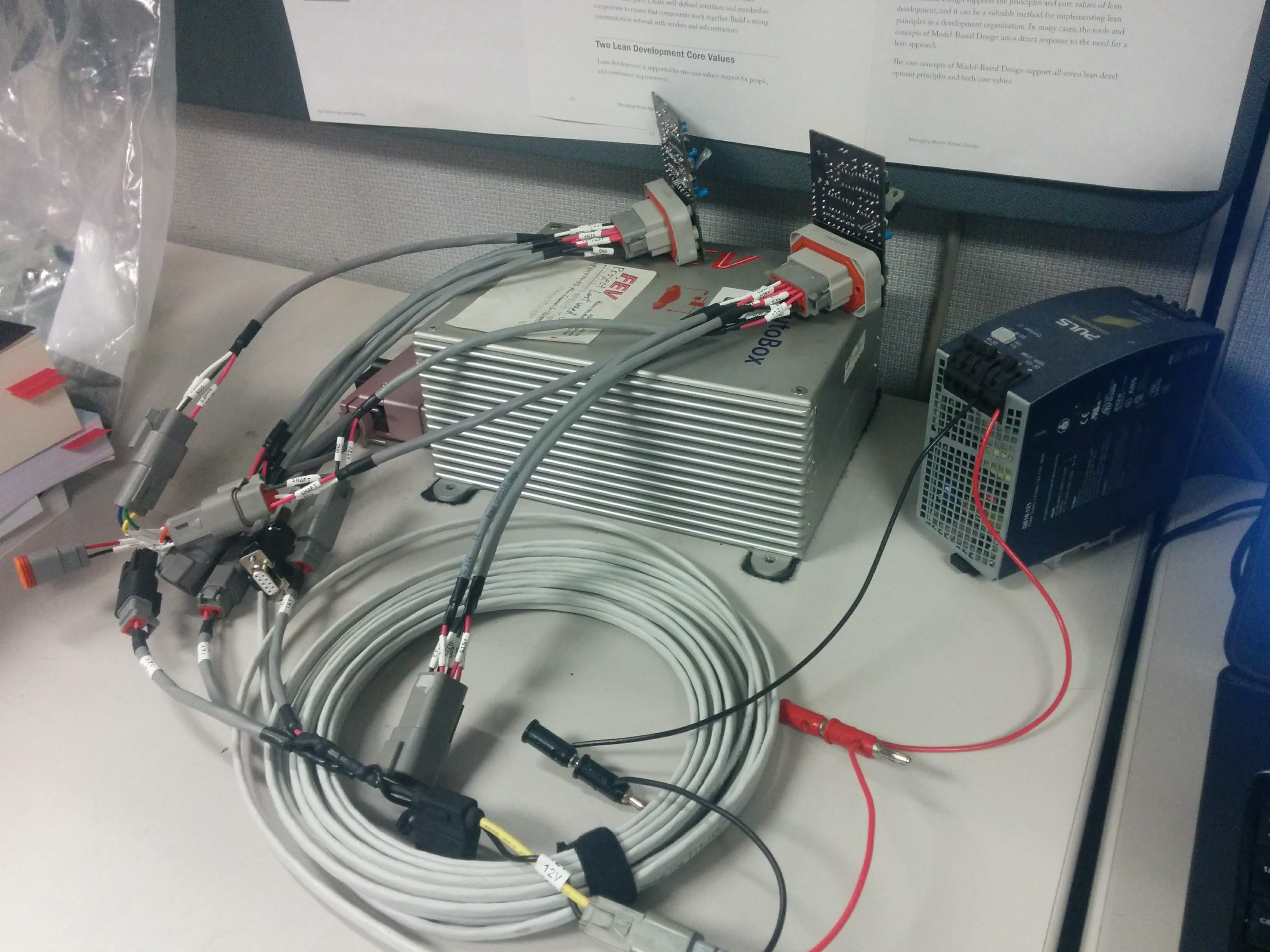
The following section is a real world application of this demodulation method on a past project. This circuit was constructed to measure the position of two resolvers in a 2018 Infinity QX50. This vehicle featured a unique feature - variable compression ratio. The compression ratio was controlled by an additional linkage, which was driven by a 12V motor. The output shaft of the motor traveled over only a very small arc. Within the motor was a very large reduction strain wave gearbox. The motor used 2 resolvers - One mounted directly at the motor, to be used by its FOC for commutation, and another at the final output, used to interpret the compression ratio.

FEV North America was benchmarking this vehicle for a customer project. During benchmarking, additional instrumentation is added to the vehicle in order to record more information. Measuring the compression ratio actuator was a critical item. This resolver demodulator circuit was made in part of a project to measure the position of the actuator, with only minimal changes to the factory wiring harness. A dSPACE MicroAutoBox was then used to track the position of both resolvers, and report compression ratio at a high rate and resolution.

Here is the schematic of the circuit which was used.

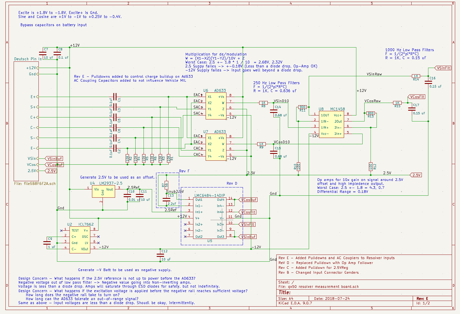
The AD633 is an analog multiplier, which implemented \(C \cdot \sin(\theta)\) and \(C \cdot \cos(\theta)\)
To the right of the AD633 are passive low pass filters (R8, C14, R9, C15), used to remove the \(2f_c\) content from the multiplied signals.
To the right of the low pass filters is a MC1458 op-amp, configured to do a 10x multiplication. The AD633 performs multiplication of inputs, but also divides by 10, so this undoes that operation.
To the right of the MC1458 op-amp are additional filters to remove high frequency noise (R14, C16, R15, C17)
Below the AD633s is an LMC6484, a set of op-amps to perform a few tasks. They buffer the output signals which acts as a protection in case the outputs were ever shorted. The second function is to buffer the 2.5V reference.
To the left of the LMC6484 is an LM2937-2.5 which creates a 2.5V reference. This signal is used by the AD633 to act as the "center" value that the output revolves around.
Next to the LM2937 is a ICL7661 which is a charge pump used to create a negative voltage reference to be used by the AD633s.
The far-most left point is a 12 Pin Deutsch connector, used to bring in power and the input signals along with connections for output signals.
Between the Deutsch connector and the AD633s are additional RCs. The capacitors were added to make it so that only AC signals were passed through. While prototyping, it was discovered that connecting the AD633s directly to the harness would create an issue that would trigger the check engine light. Adding capacitors made it so that only the AC content of the signals was passed through, which fixed the issue. The resistors were added to ensure that none of the signals going into the AD633 remained floating.
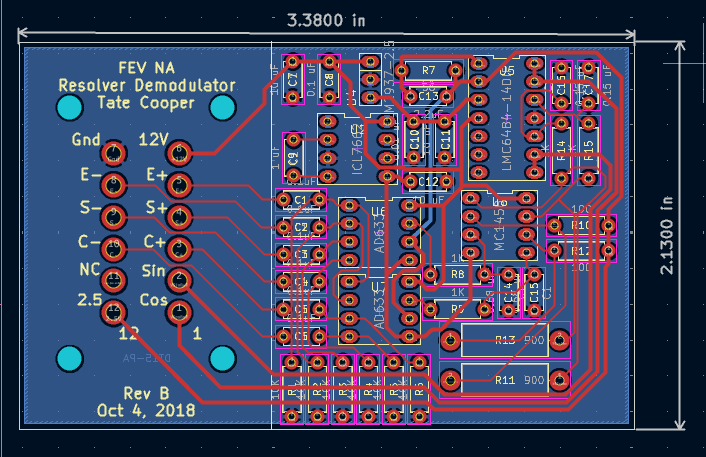
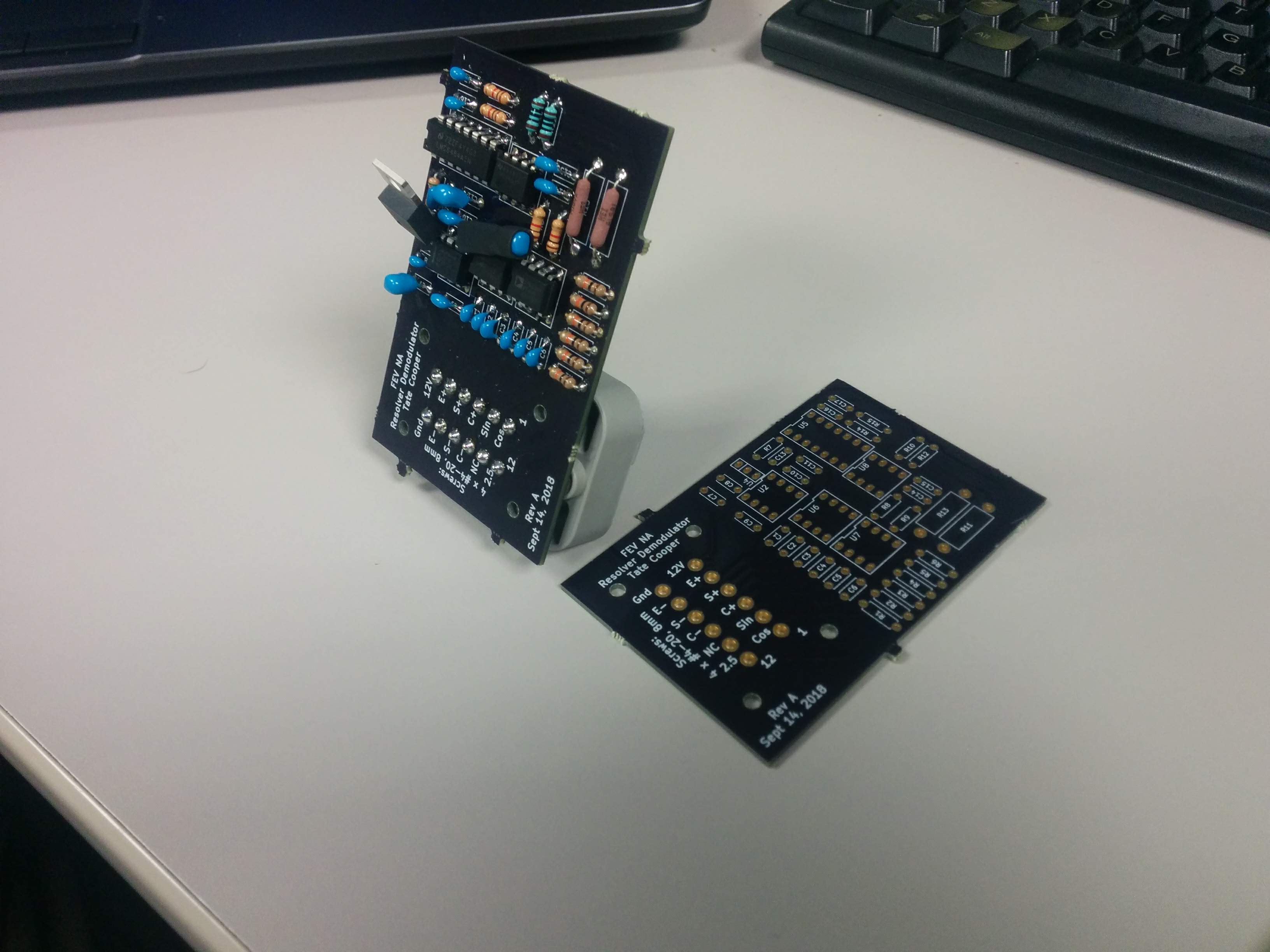
All the parts were selected to be through-hole for simplicity and ease of assembly.

Two boards wired up with a dSPACE MicroAutoBox

Building a Resolver Observer

This section documents a design process for a resolver tracker or resolver observer which does not depend on control theory. It starts simple, and iterates by fixing issues with previous versions.

To begin, the following code plots just the position and the demodulated signals, plus some noise.

using ModelingToolkit, OrdinaryDiffEq, Plots
using DataInterpolations, Distributions
gr()
using ModelingToolkit: t_nounits as t, D_nounits as D

@variables begin
    theta(t)
    we(t) 
    sine_sig(t)
    cosine_sig(t)
end

@parameters begin
    we_cmd
end

shaft_speed = 1000
num_cyc = 5
Ts = 1e-4
per = num_cyc * (2*pi/shaft_speed)

t_vec = collect(0:Ts:per)
noise1 = rand(Normal(0, 0.05), length(t_vec))
noise2 = rand(Normal(0, 0.05), length(t_vec))

noise_itp_sine = LinearInterpolation(noise1, t_vec, 
    extrapolation=ExtrapolationType.Periodic)
noise_itp_cosine = LinearInterpolation(noise2, t_vec, 
    extrapolation=ExtrapolationType.Periodic)

@named resolver = System(
    Equation[D(theta) ~ we
        we ~ we_cmd
        sine_sig ~ sin(theta) + noise_itp_sine(t)
        cosine_sig ~ cos(theta) + noise_itp_cosine(t)], 
    t
)
resolver = structural_simplify(resolver)

u0 = [
    resolver.theta => 0.0
    we_cmd => shaft_speed
]

prob = ODEProblem(resolver, u0, (0, per))
sol = solve(prob, Tsit5(), saveat=Ts)

p_demod = plot(sol[t], sol[resolver.sine_sig], label="Demod. Sin", 
    ylabel = "V")
plot!(p_demod, sol[t], sol[resolver.cosine_sig], label="Demod. Cos")

p_angle = plot(sol[t], mod.(sol[resolver.theta], 2*pi), label="Ang", 
    xlabel="Time [s]", ylabel = "rad")

plot(p_demod, p_angle, layout=(2,1), link=:x)

A simple approach is to directly use \(\arctan\) and take the derivative to get velocity.

\[\theta = \arctan\left(\dfrac{\sin(\theta)}{\cos(\theta)}\right)\] \[\omega = \dfrac{d}{dt}(\theta)\]

@variables begin
    est_theta(t)
    est_we(t)
end

@named resolver = System(
    Equation[D(theta) ~ we
        we ~ we_cmd
        sine_sig ~ sin(theta) + noise_itp_sine(t)
        cosine_sig ~ cos(theta) + noise_itp_cosine(t) 
        est_theta ~ atan(sine_sig, cosine_sig) # New!
        est_we ~ D(est_theta)], # New
    t)

This approach works, but it's far from perfect. The velocity estimate is quite noisy, a usual properly of taking a derivative directly. A simple filter on velocity can be used to clean it up.

function low_pass_filter(;name) #New
    @variables begin
        u(t)
        y(t)=0.0
    end
    @parameters begin
        bw = 300.0*2*pi
    end
    System(Equation[D(y) ~ (u - y) * bw], t, name=name)
end
@named lpf = low_pass_filter()
@variables filt_we(t)
resolver = compose(System(
    Equation[D(theta) ~ we
        we ~ we_cmd
        sine_sig ~ sin(theta) + noise_itp_sine(t)
        cosine_sig ~ cos(theta) + noise_itp_cosine(t) 
        est_theta ~ atan(sine_sig, cosine_sig)
        est_we ~ D(est_theta) 
        filt_we ~ lpf.y # New
        est_we ~ lpf.u], # New
    t, name=:resolver), lpf)

The filtered velocity is an improvement, but there is a large delay due to the filter which will cause slope of position and velocity to not agree.

An alternative is to apply the filter to the position, and then extract velocity from the filter. The low pass filter as a single line looks like

\[\dfrac{dy}{dt} = (u - y) \cdot k\]

If where \(u\) is the input and \(y\) is the output. When the filter is applied on a position signal, the output \(y\) will be a position, then \(\frac{dy}{dt}\) will be the velocity. But without directly taking a derivative. Instead, by traveling backwards through an integrator, the derivative can be calculated.

@named resolver = System(
    Equation[D(theta) ~ we
        we ~ we_cmd
        sine_sig ~ sin(theta) + noise_itp_sine(t)
        cosine_sig ~ cos(theta) + noise_itp_cosine(t)], 
    t
)
@variables begin
    theta_hat(t)
    we_hat(t)
end
@parameters begin
    k = 300*2*pi
end
@named simple_estimation = System(
    Equation[theta ~ atan(sine_sig, cosine_sig), 
        we_hat ~ (theta - theta_hat) * k, 
        D(theta_hat) ~ we_hat], t)
combined = compose(System([
    resolver.sine_sig ~ simple_estimation.sine_sig
    resolver.cosine_sig ~ simple_estimation.cosine_sig
    ], t; name=:combined), 
    resolver, simple_estimation)

This does make it so that velocity and position are related by a derivative. But there is now a large jump every time angle wraps around.

A simple way to fix this is to replace the error calculation in the low pass filter with

\[e = \text{mod}(u - y + \pi, 2\cdot\pi) - \pi\]

This will bound the error between \(-\pi\) and \(\pi\), but also make it so that when there is a roll-over at \(0\) or \(2\pi\), the error remains small, and there is no discontinuity.

While this does eliminate the discontinuity, it does create a phenomenon where angle is constantly increasing beyond \(2\pi\). However, this is correct behavior. For the sensor output, there's no difference between \(0\), \(2\pi\), \(4\pi\), etc.. For the sake of plotting, \(\text{mod}(x, 2\pi)\) will be used to constrain the plots. For electrical machines in practice, usually \(0\) to \(2\pi\) over the electrical period is needed for commutation.

As a specific note, it is worth writing a custom integrator for embedded targets which integrates velocity and outputs a position which ranges from \(0\) to \(2\pi\), automatically wrapping it's output. This prevents angle from having to accumulate forever, which could lead to floating point issues for applications which must run indefinitely. At the time of writing, it is possible to write the same sort of integrator using ModelingToolkit, but it is enough to use \(\text{mod}\) in the plots since simulations are short. Of course, if the absolute angle is what is required, and that angle is reasonably well bounded, then skip this advice.

There is one more change that can be made, which will help down the road, but also for computational performance - the removal of \(\arctan\).

Currently, this system works by

Calculating an angle with \(\arctan\)
Passing that angle into a low pass filter
Velocity is calculated using an error in the filter
Filtered Position is calculated by integrating that velocity

Within step 3, a position error is being calculated. An alternative way to calculate that error is by using

\[e \approx \sin(u - y)\]

This approximation will work as long as the filter is tuned appropriately. This also allows the sine function to be exchanged with any trig identity, including

\[\sin(\theta - \phi) = \sin(\theta) \cdot \cos(\phi) - \cos(\theta) \cdot \sin(\phi) \]

A benefit of this is that a resolver already reports \(\sin(\theta)\) and \(\cos(\theta)\), so there is no need to calculate them. This replaced one calculation using \(\arctan\) with one \(\sin\) and one \(\cos\). The end result is mostly the same. One of the position estimates from the simple_estimation system is also gone.

Now the most apparent issue is that there is a steady state error, and there is still no acceleration estimate. The steady state error is a particular issue for using the trig-identity error, since it depends on the angle error being small to be accurate.

Addressing steady state error is normally done by adjusting the controller, but there is no explicit controller in this system. But within the low pass filter, there is a calculation for an error, and it is scaled with some gain to achieve some bandwidth, meaning this has been subtly using a proportional controller.

The solution is easy then! Like with most proportional controllers, there is some steady state error, and it can be fixed by adding an integral element. An alternative is to increase the proportional gain, but that will never fix the steady state error, just make it smaller, along with making the system more sensitive to noise.

@variables begin
    theta_hat(t)
    we_hat(t)
    ang_error(t)
    int_state(t)=0
end
@parameters begin
    kp = 300*2*pi
    ki = kp*300/5*2*pi
end
@named PI_estimator = System(
    Equation[
        ang_error ~ sine_sig * cos(theta_hat) - sin(theta_hat) * cosine_sig
        D(int_state) ~ ki * ang_error
        we_hat ~ ang_error * kp + int_state
        D(theta_hat) ~ we_hat], t)

combined = compose(System([
    resolver.sine_sig ~ PI_estimator.sine_sig
    resolver.cosine_sig ~ PI_estimator.cosine_sig
    ], t; name=:combined), 
    resolver, PI_estimator)

With that change, the position estimate now has zero steady state error for constant velocity. This doesn't fix all issues with steady state errors - there will still be a steady state position error during acceleration, but this tends to be very small at the acceleration rates that can be realistically achieved with motors in real world applications.

Next on the to-do list is to get an acceleration estimate. Similar to how the velocity estimate by going backwards through an integrator, an acceleration estimate can be found by going backwards through one which is outputting velocity.

The change is simple - Instead of the feedback element going into a single integrator, it will go into a double integrator. The final output will be position, due to the closed loop. Going backwards through the last integrator will give velocity. Since the first integrator is outputting velocity, it's input will be an acceleration estimate.

If this change is blindly applied to the simulation, things don't go well.

@variables begin
    theta_hat(t)
    we_hat(t)
    alpha_hat(t)
    ang_error(t)
    int_state(t)=0
end
@named PI_2ndOrd_estimator = System(
    Equation[
        ang_error ~ sine_sig * cos(theta_hat) - sin(theta_hat) * cosine_sig
        D(int_state) ~ ki * ang_error
        alpha_hat ~ ang_error * kp + int_state
        D(we_hat) ~ alpha_hat
        D(theta_hat) ~ we_hat], t)

This response almost looks like a software bug, that the position and velocity aren't moving at all. They are, they're just making very small changes. The issue is that the gains weren't updated accordingly when the model was changed. It also doesn't help that the simulation asks the resolver to pick up such a large speed change.

One indication that something has to be changed is looking at the closed loop transfer function. The loop with a single integrator was

\[\dfrac{\hat \theta(s)}{\theta(s)} = \dfrac{k_p + k_i/s}{s + k_p + k_i/s}\]

and the new one is

\[\dfrac{\hat \theta(s)}{\theta(s)} = \dfrac{k_p + k_i/s}{s^2 + k_p + k_i/s}\]

The characteristic polynomials have changed, which necessitates some retuning.

Another sign that the gain is part of the problem is looking at units. The old proportional gain had units of \(sec^{-1}\). Error was position in \(rad\) and the output was velocity \(rad/s\) so the units for \(k_p\) would have to be \(sec^{-1}\). In this new configuration, the controller takes in position but outputs acceleration in \(rad/s^2\), so the units for \(k_p\) are now \(sec^{-2}\). If there was a derivative gain, that would take in velocity error and output acceleration, which would have units of \(sec^{-1}\).

In that case, a derivative element can be added, and the old proportional gain will become the derivative gain.

@parameters begin
    kd = 300*2*pi
    kp = kd*300/5*2*pi
    ki = kp*300/5^2*2*pi
end
@named PID_2ndOrd_estimator = System(
    Equation[
        ang_error ~ sine_sig * cos(theta_hat) - sin(theta_hat) * cosine_sig
        D(int_state) ~ ki * ang_error
        alpha_hat ~ ang_error * kp + int_state + D(ang_error) * kd
        D(we_hat) ~ alpha_hat
        D(theta_hat) ~ we_hat], t)

This works! And all the desired outputs exist.

This solution required taking a derivative directly in the feedback controller, which was considered undesirable before. The design can be changed slightly so that there is derivative action without taking a derivative. By changing where the derivative action is included, the same position response can be achieved without taking a derivative.

Consider the open loop equation for the system right now

\[\theta = \dfrac{1}{s} \cdot \dfrac{1}{s} \cdot \left(k_p + k_i \cdot \dfrac{1}{s} + k_d \cdot s \right) \cdot e \]

If the derivative action \(k_d \cdot s\) is un-distributed from the parenthesis, once multiplied with the integrator, the derivative and integrator would cancel.

\[\theta = \dfrac{1}{s} \cdot \left(\dfrac{1}{s} \cdot \left(k_p + k_i \cdot \dfrac{1}{s} \right) + \dfrac{1}{s} \cdot k_d \cdot s\right) \cdot e = \dfrac{1}{s} \cdot \left(\dfrac{1}{s} \cdot \left(k_p + k_i \cdot \dfrac{1}{s} \right) + k_d\right) \cdot e\]

In code, this means that the sum of the PI action goes into the first integrator, and then the D action is added to that before going into the second integrator.

@variables begin
    theta_hat(t)
    we_hat_smooth(t)
    we_hat_course(t)
    alpha_hat(t)
    ang_error(t)
    int_state(t)=0
end
@named PID_2ndOrd_estimator = System(
    Equation[
        ang_error ~ sine_sig * cos(theta_hat) - sin(theta_hat) * cosine_sig
        D(int_state) ~ ki * ang_error
        alpha_hat ~ ang_error * kp + int_state
        D(we_hat_smooth) ~ alpha_hat
        we_hat_course ~ we_hat_smooth + kd * ang_error
        D(theta_hat) ~ we_hat_course], t)

With this change, there are two potential velocity estimates to use, one from before including the derivative action and one from after. The one after will be a true derivative with respect to position. The one before will not be a true derivative, but will also lack the noise added by the derivative action. This also changes the frequency content of the acceleration estimate, which is no longer directly impacted by the derivative at all.

Changing the location where the derivative is included also changes the dynamic behavior of the acceleration estimate. It removes noise from it, at the expense of having a slower response. Another compromise with this change is that it doesn't ensure that acceleration to position are related exactly by two derivatives.

At this point, the resolver observer is essentially finished. The following is an entire code snippet that could be run to recreate the final version.

using ModelingToolkit, OrdinaryDiffEq, Plots
using DataInterpolations, Distributions
gr()
using ModelingToolkit: t_nounits as t, D_nounits as D

@variables begin
    theta(t)
    we(t) 
    sine_sig(t)
    cosine_sig(t)
end

shaft_speed = 1000
num_cyc = 5
noise_freq = 1e-4
per = num_cyc * (2*pi/shaft_speed)

t_vec = collect(0:noise_freq:per)
noise1 = rand(Normal(0, 0.05), length(t_vec))
noise2 = rand(Normal(0, 0.05), length(t_vec))

noise_itp_sine = LinearInterpolation(noise1, t_vec, 
    extrapolation=ExtrapolationType.Linear)
noise_itp_cosine = LinearInterpolation(noise2, t_vec, 
    extrapolation=ExtrapolationType.Linear)

@parameters we_cmd=shaft_speed
@named dynamic_shaft = System(
    Equation[D(we) ~ (we_cmd - we) * k, 
        D(theta) ~ we], t)

@named resolver = System(
    Equation[
        sine_sig ~ sin(theta) + noise_itp_sine(t)
        cosine_sig ~ cos(theta) + noise_itp_cosine(t)], 
    t
)

@variables begin
    theta_hat(t)
    we_hat_smooth(t)
    we_hat_course(t)
    alpha_hat(t)
    ang_error(t)
    int_state(t)=0
end
@parameters begin
    kd = 300*2*pi
    kp = kd*300/5*2*pi
    ki = kp*300/5^2*2*pi
end

@named PID_2ndOrd_estimator = System(
    Equation[
        ang_error ~ sine_sig * cos(theta_hat) - sin(theta_hat) * cosine_sig
        D(int_state) ~ ki * ang_error
        alpha_hat ~ ang_error * kp + int_state
        D(we_hat_smooth) ~ alpha_hat
        we_hat_course ~ we_hat_smooth + kd * ang_error
        D(theta_hat) ~ we_hat_course], t)

combined = compose(System([
    resolver.sine_sig ~ PID_2ndOrd_estimator.sine_sig
    resolver.cosine_sig ~ PID_2ndOrd_estimator.cosine_sig
    resolver.theta ~ dynamic_shaft.theta
    ], t; name=:combined), 
    resolver, PID_2ndOrd_estimator, dynamic_shaft)

combined = structural_simplify(combined)

u0 = [
    PID_2ndOrd_estimator.theta_hat => 0.0
    PID_2ndOrd_estimator.we_hat_smooth => 0.0
    dynamic_shaft.we => shaft_speed
    dynamic_shaft.theta => 0.0
    dynamic_shaft.k => 500
]

prob = ODEProblem(combined, u0, (0, per))
sol = solve(prob, Tsit5(), saveat=noise_freq)

p_demod = plot(sol[t], sol[resolver.sine_sig], 
    label="Demod. Sine", ylabel="V")
plot!(p_demod, sol[t], sol[resolver.cosine_sig], 
    label="Demod. Cosine")

p_angle = plot(sol[t], mod.(sol[resolver.theta], 2*pi), 
    label="Ang")
plot!(p_angle, sol[t], sol[PID_2ndOrd_estimator.theta_hat], 
    label="Est Ang, Filt")

p_ang_err = plot(sol[t], 
    mod.(sol[resolver.theta] - sol[PID_2ndOrd_estimator.theta_hat] .+ pi, 2*pi) .- pi, 
    label="Ang Err")

p_vel = plot(sol[t], sol[dynamic_shaft.we], 
    label="Vel")
plot!(p_vel, sol[t], sol[PID_2ndOrd_estimator.we_hat_smooth], 
    label="Est Vel, smooth")
plot!(p_vel, sol[t], sol[PID_2ndOrd_estimator.we_hat_course], 
    label="Est Vel, course")

p_accel = plot(sol[t], sol[PID_2ndOrd_estimator.alpha_hat], 
    xlabel="Time [s]", label="Est. Accel")

plot(p_demod, p_angle, p_ang_err, p_vel, p_accel, layout=(5,1), link=:x)

Speeding Up with Theory

Control theory offers some ways to speed up this design process, especially steady state error analysis.

In the previous section, the steady state tracking error was addressed by adding an integral gain. Using steady state error analysis, it would have been possible to see this was an issue immediately instead of once getting to simulation.

In steady state error analysis, it is possible to examine what the final error value will be as time stretches out to infinity. The process is

Come up with the transfer function between the input \(r\) and the error \(e\)
Multiply by the appropriate shape of \(r\) (impulse, step, ramp, etc.)
Use the final value theorem to see what the error \(e\) will be

As an example, the low pass filter design can be used, which looked like a true integrator plant with a proportional gain.

\[G = \dfrac{1}{s}\] \[K = k_p\]

The error \(e\) can be calculated using

\[e = r - y = r - G \cdot K \cdot e = r - \dfrac{k_p}{s}\]

yielding the transfer function

\[e = \dfrac{s}{s + k_p} \cdot r\]

If the input \(r\) is a step

\[e = \dfrac{s}{s + k_p} \cdot \dfrac{1}{s}\]

The Final Value Theorem stablishes that

\[\lim\limits_{t\rightarrow\infty} f(t) = \lim\limits_{s\rightarrow 0} s \cdot F(s)\]

So the final value for error of this system with a step input is

\[e_{ss} = \lim\limits_{s\rightarrow 0} \left(s \cdot \dfrac{s}{s + k_p} \cdot \dfrac{1}{s}\right) = 0\]

so there's no steady state error!

However when operating at speed, position is not a step, but a ramp. For a ramp input

\[e = \dfrac{s}{s + k_p} \cdot \dfrac{1}{s^2}\] \[e_{ss} = \lim\limits_{s\rightarrow 0} \left(s \cdot \dfrac{s}{s + k_p} \cdot \dfrac{1}{s^2}\right) = \dfrac{1}{k_p} \]

This indicates that there will be a steady state error. As mentioned earlier, the error can be reduced by increasing the proportional gain, but it will not be zero.

By changing to a PI controller with a single integrator tracking a ramp input

\[e = (r - y) = r - G \cdot K \cdot e = r - \dfrac{k_p + k_i/s}{s}\] \[e = \dfrac{s}{s + k_p + k_i/s} \cdot r\] \[e_{ss} = \lim\limits_{s\rightarrow 0} \left(s \cdot \dfrac{s}{s + k_p + k_i/s} \cdot \dfrac{1}{s^2}\right) = 0 \]

This shows that there will be no steady state error.

There is also a chance to review why a PI controller was insufficient when using two integrators. Even though the performance was not stellar, the closed loop transfer function yields some information that makes it obvious that a derivative gain would be needed.

The starting controller was

\[K = k_p + k_i/s\]

and the plant

\[G = \dfrac{1}{s^2}\]

The closed loop transfer function is then

\[\dfrac{y}{r} = \dfrac{k_p + k_i/s}{s^2 + k_p + k_i/s}\]

The characteristic polynomial is completely devoid of a term for \(s\). This means that the polynomial can only be broken down into

\[P = (s^2 + \omega_n^2) \cdot (s + \lambda)\]

This would create an oscillator! Not the desired intent. Changing to a PID yields

\[\dfrac{y}{r} = \dfrac{k_d \cdot s + k_p + k_i/s}{s^2 + k_d \cdot s + k_p + k_i/s}\]

This allows for the poles to be placed at any location.

Handling Imperfect Parameters

Up to this point it was assumed that the demodulated signals were exactly

\[V_{demod,sin} = \sin(\theta) \] \[V_{demod,cos} = \cos(\theta) \]

In practice, this isn't the case. While the shapes of the \(\sin\) and \(\cos\) waveforms are likely to look close to their ideal trig functions, it is common to have sort of scaling and offset error. It is also possible that \(\sin\) and \(\cos\) are not exactly \(\pi/2\) apart, sometimes called an orthogonality error. Better models for the functions might be

\[V_{demod,sin} = k_s \cdot \sin(\theta) + g_s\] \[V_{demod,cos} = k_c \cdot \cos(\theta + \phi) + g_c\]

There may also be no guarantee that these parameters are constant and my vary over time.

Running the same tracking system as before, but with some parameter errors yields the following.

@parameters begin
    sin_gain = 1.05
    sin_ofs = -0.02
    cos_gain = 0.98
    cos_ofs = 0.04
    cos_ortho = pi/20
end

@named imperfect_resolver = System(
    Equation[
        sine_sig ~ sin_gain * sin(theta) + sin_ofs + noise_itp_sine(t)
        cosine_sig ~ cos_gain * cos(theta + cos_ortho) + 
            cos_ofs + noise_itp_cosine(t)], 
    t
)

The most substantial change is that the position signal and its derivatives are no longer smooth. With a long simulation, and a plot of estimated position versus actual, it can be seen that there are now harmonics that are a function of position.

These same harmonics show up in the FFT of the velocity estimate. They also show up in the FFT of the position estimate, but the sawtooth shape makes the FFT of position more difficult to parse.

using FFTW
N = length(sol[PID_2ndOrd_estimator.we_hat_course])
Fs = 1/Ts
delta_f = Fs / N
F_vec = (0:1:(N-1)) .* delta_f
complex = fft(sol[PID_2ndOrd_estimator.we_hat_course])
mag = abs.(complex)
phase = angle.(complex)

p1 = scatter(F_vec[2:end], mag[2:end], xlabel="Frequency [Hz]", ylabel="Magnitude", 
    xscale=:log10,
    xlim=(F_vec[2], 5e3), 
    label="Velocity FFT", 
    legend=:topleft)
vline!(p1, [shaft_speed/2/pi], label="Electrical Frequency")
vline!(p1, [2 * shaft_speed/2/pi], label="2 * Electrical Frequency")

The parameters create harmonics which are first order and second order harmonics with position, which matches the behavior seen in the position error plot.

To fix these, it is necessary to come up with improve estimates of what the \(\sin\) and \(\cos\) signals actually are. Online Parameter Estimators from adaptive controls are a good fit for this, since fitting sine and cosine functions is an introductory-level problem in many adaptive controls books (e.g. Ioannou and Sun - Robust Adaptive Controls, Example 4.3.1).

For modeling the sine function, the following equations can be used to model the demodulated sine signal.

\[z_{sin} = \theta_{sin}^T \cdot \psi_{sin}\] \[\theta_{sin} = \begin{bmatrix}\hat k_s \\ \hat g_s\end{bmatrix}\] \[\psi_{sin} = \begin{bmatrix}\sin(\hat \theta) \\ 1\end{bmatrix}\]

The position estimate \(\hat \theta\) is the position estimated by the resolver observer, since there is no direct access to the true position.

For adaption, Instantaneous Cost Gradient Descent can be used. It is simple, and this problem may not warrant anything more complicated than this.

\[e = \dfrac{V_{demod,sin} \cdot \lambda}{s + \lambda} - \theta_{sin}^T \cdot \left(\dfrac{\lambda}{s + \lambda} \cdot \psi_{sin}\right)\] \[\dfrac{d\theta_{sin}}{dt} = k \cdot e \cdot \psi_{sin}\]

The filtering may not be necessary. Filtering is normally used in adaptive control problems when higher order derivatives are needed, which isn't the case here. However, filtering can provide some additional tuning parameters besides just adaption gain.

Normalization can be skipped. There is good confidence about the range of the inputs and the dynamics of the resolver observer.

The ModelingToolkit code is

function low_pass_filter(;name)
    @variables begin
        u(t)
        y(t)=0.0
    end
    @parameters begin
        lambda = 15.0
    end
    System(Equation[D(y) ~ (u - y) * lambda], t, name=name)
end
function SineAdpt(;name)
    @variables begin
        theta(t)
        sine_sig(t)
        error(t)
        params(t)[1:2]
        regressor(t)[1:2] #psi
        est_true(t)
    end
    @parameters begin
        k[1:2]
    end
    @named lpf1 = low_pass_filter()
    @named lpf2 = low_pass_filter()
    return compose(System(
        Equation[
            lpf1.u ~ sin(theta)
            lpf2.u ~ sine_sig

            regressor ~ [lpf1.y, 1.0]
            error ~ lpf2.y - params' * regressor
            D(params) ~ k .* error .* regressor
            est_true ~ params' * [sin(theta), 1]            
        ], t; name=name), lpf1, lpf2)
end

Repeating this setup for cosine, we have

\[z_{cos} = \theta_{cos}^T \cdot \psi_{cos} \] \[\theta_{cos} = \begin{bmatrix}\hat k_{c1} \\ \hat k_{c2} \\ \hat g_c\end{bmatrix} \] \[\psi_{cos} = \begin{bmatrix}\sin(\hat \theta) \\ \cos(\hat \theta)\\ 1\end{bmatrix} \]

The reason that cosine is set up different from sine is that the cosine function is going to be allowed to shift its phase to account for any orthogonality error. A phase adaption cannot be included in both signals because it will create an issue where both sine and cosine signals can shift far from their ideal model, which can violate the assumptions made in the resolver observer's error calculation.

\[e = \dfrac{V_{demod,cos} \cdot \lambda}{s + \lambda} - \theta_{cos}^T \cdot \left(\dfrac{\lambda}{s + \lambda} \cdot \psi_{cos}\right)\] \[\dfrac{d\theta_{cos}}{dt} = k \cdot e \cdot \psi_{cos}\]

And again, the code is

function CosineAdapt(;name)
    @variables begin
        theta(t)
        cosine_sig(t)
        error(t)
        params(t)[1:3]
        regressor(t)[1:3] #psi
        est_true(t)
    end
    @parameters begin
        k[1:3]
    end
    @named lpf1 = low_pass_filter()
    @named lpf2 = low_pass_filter()
    @named lpf3 = low_pass_filter()
    return compose(System(
        Equation[
            lpf1.u ~ sin(theta)
            lpf2.u ~ cos(theta)
            lpf3.u ~ cosine_sig

            regressor ~ [lpf1.y, lpf2.y, 1.0]
            error ~ lpf3.y - params' * regressor
            D(params) ~ k .* error .* regressor
            est_true ~ params' * [sin(theta), cos(theta), 1]            
        ], t; name=name), lpf1, lpf2, lpf3)
end

The final detail is to close the loop. The adaptions take in tracker estimated position, and the tracker now needs to take in these adapted models in its feedback path. This is an important detail. The purpose of the adaption isn't to come up with some way to remove the imperfections from the measured signals. Those are left as they are. Instead, the goal is to make it so that the tracker knows that the signals are somewhat defective.

This is another one of the reasons that using the trig identity for the error function in the tracker is preferable - It allows the flexibility to replace \(\sin(\hat \theta)\) and \(\cos(\hat \theta)\) with any alternative. This does mean that the error equation will no longer be a perfect trig identity, but that was still only an approximation.

@variables begin
    cos_feedback(t) #Connected to CosAdpt.est_true
    sin_feedback(t) #Connected to SinAdpt.est_true
end
@named PID_2ndOrd_estimator = System(
    Equation[
        ang_error ~ sine_sig * cos_feedback - sin_feedback * cosine_sig
        D(int_state) ~ ki * ang_error
        alpha_hat ~ ang_error * kp + int_state
        D(we_hat_smooth) ~ alpha_hat
        we_hat_course ~ we_hat_smooth + kd * ang_error
        D(theta_hat) ~ we_hat_course], t)

A final note is that the tuning gain for each adaption parameter needs to be adjusted. This can be a trail-and-error process. For this example, the gain for the offset is about \(1/1000\) of the gain used for the \(\sin\) and \(\cos\) signals.

This shows that the adaptions converge to the defective parameters specified earlier. The improvement in the angle estimation can be seen as the noise in angle estimation error decreases over time. For the cosine model, a little more effort is needed to extract the orthogonality angle and cosine magnitude error and show that the estimate did converge to the correct value.

The model used was

\[V_{demod,cos} = \begin{bmatrix}\hat k_{c1} \\ \hat k_{c2} \\ \hat g_c\end{bmatrix}^T \cdot \begin{bmatrix} \sin(\hat \theta) \\ \cos(\hat \theta) \\ 1 \end{bmatrix} = k_{c1} \cdot \sin(\hat \theta) + k_{c2} \cdot \cos(\hat \theta) + g_c = A \cdot \cos(\theta + \phi) + g_c \]

The equation above is similar to the trig identity

\[\cos(\theta + \phi) = \cos(\theta) \cdot \cos(\phi) - \sin(\theta) \cdot \sin(\phi)\]

Therefore

\[k_{c1} = -A \cdot \sin(\phi)\] \[k_{c2} = A \cdot \cos(\phi)\]

The orthogonality error can be found using

\[\phi = \arctan\left(\dfrac{A \cdot \sin(\phi)}{A \cdot \cos(\phi)}\right) = \arctan\left(\dfrac{0.14}{0.97}\right) \approx 0.14 \approx \pi/20\]

And the magnitude error can be found using

\[A = k_{c1} / \cos(\phi) \approx 0.979\]

Rotation Multiples

The previous sections assumed that the angle being reported by the resolver is the one that is needed. Usually a resolver is selected appropriately for a motor, so that the resolver angle matches the motors electrical angle. A four times resolver for an eight pole machine, a three times resolver for a six pole machine.

But this is not always the case. As an example, a six pole machine may come with a SinCos sensor which outputs two pairs of demodulated signals, one pair which is once per mechanical revolution and one pair which is twice per mechanical revolution.

To write it as some equations

\[\theta_e = 3 \cdot \theta_m\] \[\theta_{SinCos1} = \theta_m\] \[\theta_{SinCos2} = 2 \cdot \theta_m\]

The following plot shows the desired position and velocity, plus the position being reported by the once-per-mechanical sensor, and twice-per-mechanical sensor.

In the case of using just the one-per-mechanical signals, it is fairly easy to simply track the position, and multiply all the outputs by 3.

Again, as equations

\[\theta_e = 3 \cdot \theta_m = 3 \cdot \theta_{SinCos1}\]

function make_resolver(; name)
    @variables begin
        theta(t)
        sine_sig(t)
        cosine_sig(t)
    end
    t_vec = collect(0:noise_freq:per)
    noise1 = rand(Normal(0, 0.05), length(t_vec))
    noise2 = rand(Normal(0, 0.05), length(t_vec))

    noise_itp_sine = LinearInterpolation(noise1, t_vec, 
        extrapolation=ExtrapolationType.Periodic)
    noise_itp_cosine = LinearInterpolation(noise2, t_vec, 
        extrapolation=ExtrapolationType.Periodic)

    System(
        Equation[
            sine_sig ~ sin(theta) + noise_itp_sine(t)
            cosine_sig ~ cos(theta) + noise_itp_cosine(t)], 
        t; name=name)
end

function make_observer(; name)
    @variables begin
        theta_hat(t)
        we_hat_smooth(t)
        we_hat_course(t)
        alpha_hat(t)
        ang_error(t)
        int_state(t)=0
    end
    @parameters begin
        kd = 300*2*pi
        kp = kd*300/5*2*pi
        ki = kp*300/5^2*2*pi
        feedback_gain = 1
    end

    System(
        Equation[
            ang_error ~ sine_sig * cos(feedback_gain * theta_hat) - 
                sin(feedback_gain * theta_hat) * cosine_sig
            D(int_state) ~ ki * ang_error
            alpha_hat ~ ang_error * kp + int_state
            D(we_hat_smooth) ~ alpha_hat
            we_hat_course ~ we_hat_smooth + kd * ang_error
            D(theta_hat) ~ we_hat_course], t;
            name=name)
end


@named resolver_1x = make_resolver()
@named resolver_2x = make_resolver()
@named desired = make_resolver()

@named observer_1x = make_observer()

combined = compose(System([
    resolver_1x.theta ~ dynamic_shaft.theta
    resolver_2x.theta ~ dynamic_shaft.theta * 2
    desired.theta ~ dynamic_shaft.theta * 3
    observer_1x.sine_sig ~ resolver_1x.sine_sig
    observer_1x.cosine_sig ~ resolver_1x.cosine_sig
    est_des ~ 3*observer_1x.theta_hat
    est_vel ~ 3*observer_1x.we_hat_course
    ], t; name=:combined), 
    dynamic_shaft, resolver_1x, resolver_2x, desired, 
        observer_1x)

Simple and effective. But what other options are there? It sounds silly, but it's worth thinking about all the different options available.

A few options are

Addition of 1, 3 times: \(\theta_e = 3 \cdot \theta_m = (1 + 1 + 1) \cdot \theta_m = \theta_{SinCos1} + \theta_{SinCos1} + \theta_{SinCos1}\)
Multiplication of 1 by 3: \(\theta_e = 3 \cdot \theta_m = 3 \cdot \theta_{SinCos1}\)
Addition of 2 and 1: \(\theta_e = 3 \cdot \theta_m = (2 + 1) \cdot \theta_m = \theta_{SinCos2} + \theta_{SinCos1}\)
Multiplication of 2 by 3/2: \(\theta_e = 3 \cdot \theta_m = 3/2 \cdot \theta_{SinCos2}\)

First, there's addition. \(2+1=3\). By using resolvers for both the once-per-rev and the twice-per-rev, the three-pre-rev signals can be found by simply adding the outputs together.

@named resolver_1x = make_resolver()
@named resolver_2x = make_resolver()
@named desired = make_resolver()

@named observer_1x = make_observer()
@named observer_2x = make_observer()

@variables est_des(t)
combined = compose(System([
    resolver_1x.theta ~ dynamic_shaft.theta
    resolver_2x.theta ~ dynamic_shaft.theta * 2
    desired.theta ~ dynamic_shaft.theta * 3
    observer_1x.sine_sig ~ resolver_1x.sine_sig
    observer_1x.cosine_sig ~ resolver_1x.cosine_sig
    observer_2x.sine_sig ~ resolver_2x.sine_sig
    observer_2x.cosine_sig ~ resolver_2x.cosine_sig
    est_des ~ observer_1x.theta_hat + observer_2x.theta_hat # Adding position
    est_vel ~ observer_1x.we_hat_course + observer_2x.we_hat_course # Adding velocity
    ], t; name=:combined), 
    dynamic_shaft, resolver_1x, resolver_2x, desired, 
        observer_1x, observer_2x)

Another way to implement addition is to do it on the input side. The trig identity for sums and differences can be used to create \(\sin(\theta_e)\) and \(\cos(\theta_e)\) signals.

\[\sin(\alpha + \beta) = \sin(\alpha) \cdot \cos(\beta) + \cos(\alpha) \cdot \sin(\beta)\] \[\cos(\alpha + \beta) = \cos(\alpha) \cdot \cos(\beta) - \sin(\alpha) \cdot \sin(\beta)\]

Substituting in leads to

\[\sin(\theta_{SinCos1}) \cdot \cos(\theta_{SinCos2}) + \cos(\theta_{SinCos1}) \cdot \sin(\theta_{SinCos2}) = \sin(\theta_{SinCos1} + \theta_{SinCos2})\] \[\cos(\theta_{SinCos1}) \cdot \cos(\theta_{SinCos2}) - \sin(\theta_{SinCos1}) \cdot \sin(\theta_{SinCos2}) = \cos(\theta_{SinCos1} + \theta_{SinCos2})\]

which happen to be the desired signals for tracking

\[\sin(\theta_{SinCos1} + \theta_{SinCos2}) = \sin(3 \cdot \theta_m) = \sin(\theta_e)\] \[\cos(\theta_{SinCos1} + \theta_{SinCos2}) = \cos(3 \cdot \theta_m) = \cos(\theta_e)\]

combined = compose(System([
    resolver_1x.theta ~ dynamic_shaft.theta
    resolver_2x.theta ~ dynamic_shaft.theta * 2
    desired.theta ~ dynamic_shaft.theta * 3
    observer.sine_sig ~ resolver_1x.sine_sig * resolver_2x.cosine_sig + 
        resolver_1x.cosine_sig * resolver_2x.sine_sig
    observer.cosine_sig ~ resolver_1x.cosine_sig * resolver_2x.cosine_sig - 
        resolver_1x.sine_sig * resolver_2x.sine_sig
    ], t; name=:combined), 
    dynamic_shaft, resolver_1x, resolver_2x, desired, 
        observer)

This achieves similar performance, but only requires one observer instead of two. The point is that any trig identities are available for use with the demodulated signals. Addition, differences, doubling, halving, tripling, etc....

Another option is multiplication, but built into the resolver observer. Instead of multiplying the outputs from the observer, the multiplication will be placed in the feedback path of the resolver observer. The gain in the feedback path will change the output of the resolver to be a multiple of the input signals. The multiple is the inverse of the gain. Place a \(2\) in the feedback path, the output will halve. Place a \(1/3\) in the feedback path, the output will triple.

This method of multiplying supports arbitrary multiples. This means it would be possible to go from the two-per-rev signals to a three-per-rev signal, by placing \(2/3\) in the feedback path. A side effect is this changes the dynamics and requires retuning the observer gains to achieve the same performance.

@named observer_2x = make_observer()

@variables est_des(t)
combined = compose(System([
    resolver_1x.theta ~ dynamic_shaft.theta
    resolver_2x.theta ~ dynamic_shaft.theta * 2
    desired.theta ~ dynamic_shaft.theta * 3
    observer_2x.sine_sig ~ resolver_2x.sine_sig
    observer_2x.cosine_sig ~ resolver_2x.cosine_sig
    est_des ~ observer_2x.theta_hat
    est_vel ~ observer_2x.we_hat_course
    ], t; name=:combined), 
    dynamic_shaft, resolver_1x, resolver_2x, desired, 
        observer_2x)

combined = structural_simplify(combined)

u0 = [
    dynamic_shaft.we => shaft_speed
    dynamic_shaft.theta => 0.0
    dynamic_shaft.k => 300
    observer_2x.we_hat_smooth => 0.0
    observer_2x.theta_hat => 0.0
    observer_2x.feedback_gain => 2/3
]

Conclusion

Hopefully these examples have been helpful. Some of these topics are complicated, but they are all solvable problems. Demodulation can be done with even simple circuits. A resolver observer can be constructed using theory, but also with a workflow of slowly checking off objectives. Adaptive estimators can be used to help remove common imperfections online in real-time. Arbitrary multiples of rotation can be found using different methods, including combinations of sensors or changing the feedback path of the observer.

As a final note, be aware that multiple observers can be used at the same time, usually to achieve different objectives. One single design may not work for all cases. These algorithms are computationally light, which means computational cost and memory footprint is not a large concern if multiple observers need to be used. Cascading observers is also an option.

CC BY-SA 4.0 Tate Cooper. Last modified: April 01, 2026. Website built with Franklin.jl and the Julia programming language.